PyTorch Internals Blog Post
These are my notes on ezyang’s blog post on Pytorch internals.
PyTorch should be thought of as a “tensor library that supports automatic differentiation”.
The tensor data type
What exactly does the `tensor` data type provides?
Intuitively, the tensor is an n-dimensional array where each entry is
some sort of scalar, e.g. int, float64, float32, float16, etc.
In practice, a tensor consists of some data (these scalars that form the
n-dimensional array) along with some metadata which describes the size
of the tensor, the type (dtype) of the elements it contains, the
device the tensor lives in (CPU memory, CUDA memory).
There are other important metadata too. Let us discuss one of them.
How is the `tensor` data type implemented in PyTorch?
The stride tensor metadata
A tensor is a mathematical concept. But, to represent it on a computer, we must define some sort of physical representation for them.
(Explanation of strides here)
Strides are the fundamental basis of how views are provided to PyTorch users.
For instance, when you use advanced indexing to select a row of a tensor, you do not create a new tensor in memory; instead, you just return a tensor which is a new view on the underlying data. In particular, this implies that editing the tensor in the new view also modifies the original tensor. If you want to “disconnect” the view from the original tensor, you must make a copy of the view.
Another example is that of selecting a column. In this case, the stride is larger than one, indicating that you skip elements in memory to represent “moving down the rows in the same column”.
The author provides us with a stride visualizer.
Strides are behind many access patterns, such as transposing, taking the diagonal, broadcasting, rolling windows, etc.
Key take away.
The key thing to retain from this part is that we actually have two
things when dealing with tensors: the logical tensor, corresponding to
the specification of sizes, strides, offsets, defining the logical
interpretation of physical memory; and the storage, which is the
actual physical memory storing the data of the tensor, and defines the
dtype. There may be multiple logical tensors using the same storage
through different views.
Tensor operations
Let us discuss a bit on how operations on a tensor are implemented. Let
us take matrix multiplication,
torch.mm,
as an example.
When you call an operation on tensors, two dispatches happen:
-
Based on the device type and layout of the tensors: whether or not it is a CPU or CUDA tensors, and also whether or not it is a strided tensor or a sparse one. The same operation is implemented on different libraries depending on these characteristics: CPU implementation, sparse CPU implementation, CUDA implementation, XLA implementation, etc.
-
Based on the dtype of the tensors: it is simply a
switchstatement. The CPU or CUDA code that implements multiplication onfloatis different from the code from the code for multiplication ofint.
Tensor extensions
Let us briefly discuss tensor extensions. These are, for example, sparse tensors, quantized tensors, TPU tensors, batch tensors, anyway, things other than the basic strided tensors.
The holy trinity.
There are three parameters which uniquely determine what a tensor is:
-
The device: a description of where the tensor’s physical memory is actually stored, e.g. on a CPU, on an NVIDIA GPU (CUDA), or perhaps on an AMD GPU (hip), or a TPU (XLA). The distinguishing characteristic of a device is that it has its own allocator, that doesn’t work with any other device.
-
The layout: a description of how to logically interpret this physical memory. The most common layout is the strided tensor, but sparse tensors have a different layout involving a pair of tensors, one for indices, and one for data. There are other even more exotic layouts, that cannot be represented using merely strides.
-
The dtype: a description of what is actually stored inside each element of the tensor. It could be some type of
floatorint, or it could be, for example, quantized integers.
A tensor extension is obtained by extending one of these directions, or by writing a wrapper around an existing PyTorch tensor that implements your object type.
The criterion of what type of extension to choose is whether or not it will be passed on the backward pass of autograd: for instance, sparse tensors should really be an extension, and not just a wrapper, because when doing optimization we want the gradients to also be sparse.
Autograd
The author raises a very good point: if tensors were all that PyTorch offered, they would basically be a Numpy clone. The distinguishing characteristic of PyTorch when it was originally released was that it provided automatic differentiation on tensors.
What does automatic differentiation do?
The answer is that it takes the existing code for a neural network and automatically fills in the missing code that actually computes the gradients of the network.
I feel that it is important to copy the figures of the post here.
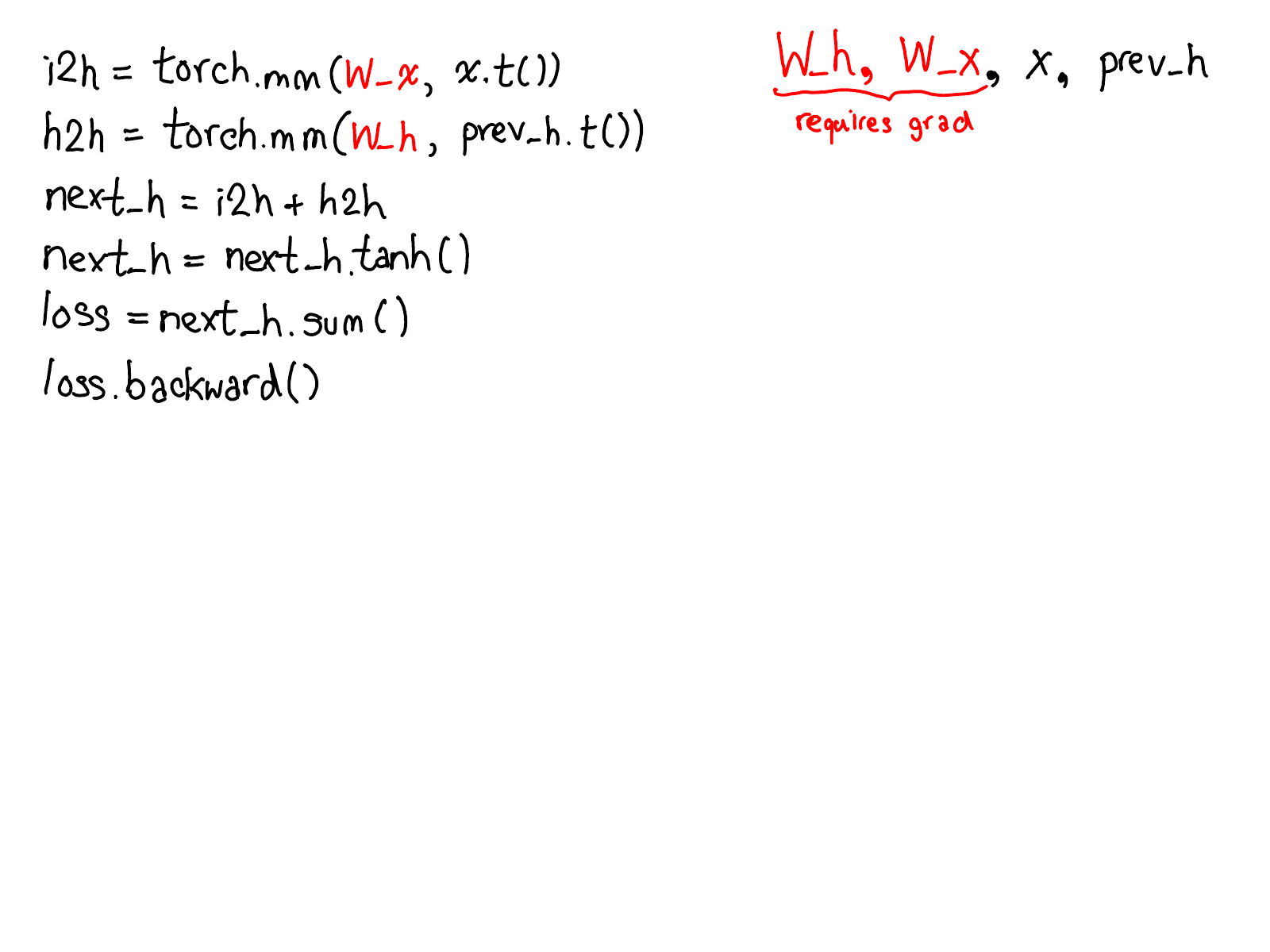
Code appearing in PyTorch.
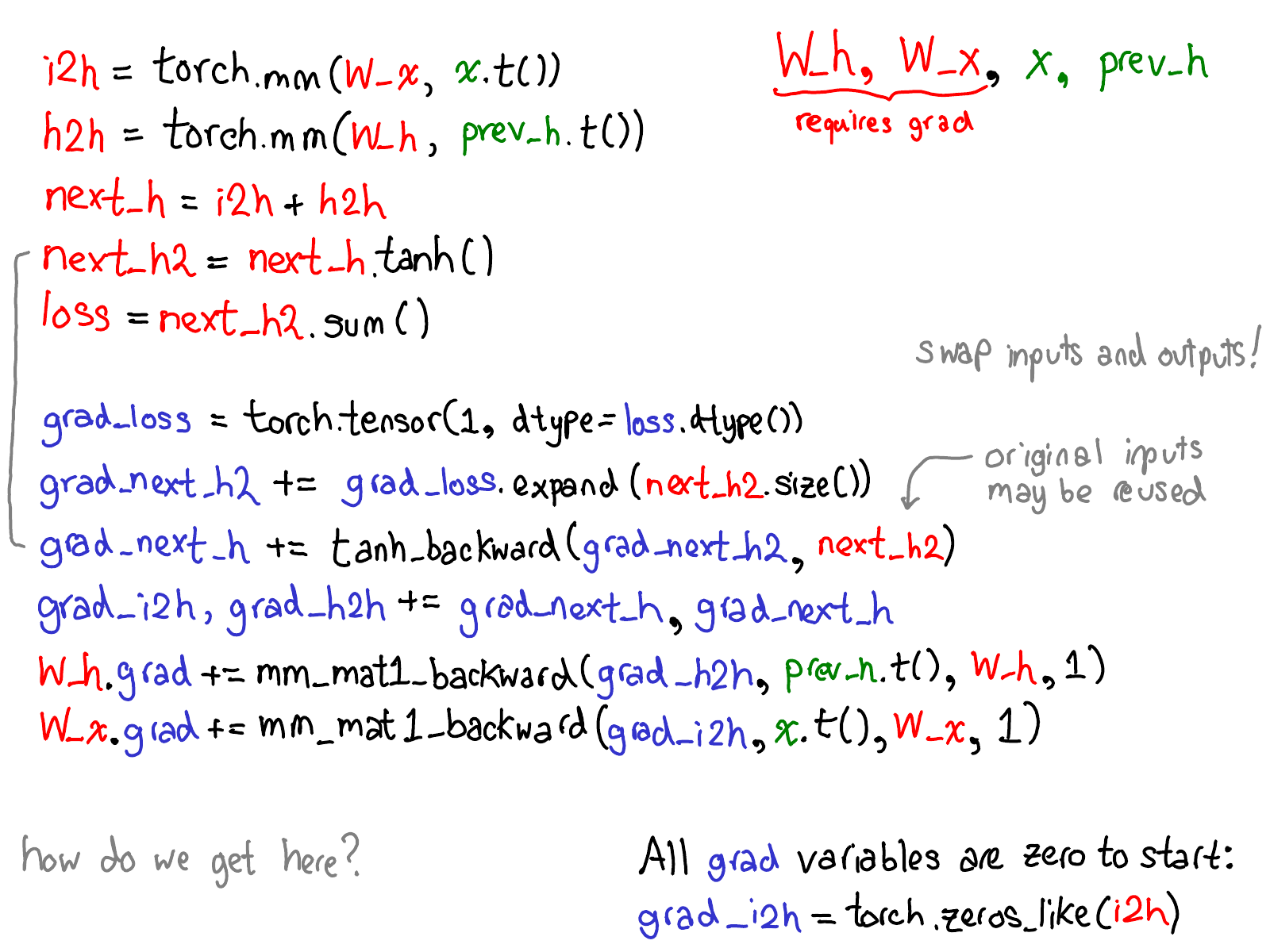
What autograd does when backward is called.
He then points out: the whole point of autograd is to do the
computation that is described by this diagram, but without actually ever
generating this source; PyTorch autograd doesn’t do a source-to-source
transformation.
I believe that the following part of the explanation is outdated, see this issue.
Confirmation: as per the PyTorch
documentation,
the Variable API is deprecated, and they are no longer necessary to use
autograd with tensors. autograd automatically supports tensors
with requires_grad=True.
To do this, we need to store more metadata when we carry out operations
on tensors. This adjusts our picture of the tensor data structure:
instead of just having a logical tensor pointing to storage, we now have
a Variable which wraps around this tensor, and also stores more
information (AutogradMeta), which is needed for performing autograd
when a user calls loss.backward() in their PyTorch script.
We also update our picture about dispatch when calling an operation on a
tensor: before we dispatch to CPU or CUDA implementations, there is
another dispatch on Variables, which is responsible for unwrapping
Variables, recording the autograd metadata, calling the underlying
implementation, then rewrapping the results into Variables and
recording the necessary autograd metadata for backwards.
The autograd engine is where the computation graph appears, but this
part in the blog post has only the slides and no write-up.
As someone put it in the PyTorch forums: “think of tensors and
Variables as the same thing; Variables are just wrappers for
tensors so you can easily auto-compute the gradients”. However, the
Variable API is now deprecated, and autograd automatically supports
tensors with requires_grad=True. To turn on gradient tracking
after creation, use tensor.requires_grad_(). Notice the trailing
underscore. To remove a tensor from the computation graph, use
.detach(). Importantly, .grad is now a built-in tensor attribute
created during .backward().
In conclusion
For the rest of the post he dives deep into the structure of the PyTorch repository, and explains how to write kernels for it, which is not something that interests us in this moment.
Other things
Here are other things I thought about when reading the article.
Trailing underscores.
One important thing to know about PyTorch is that trailing underscores
on a method e.g. add_, sin_, requires_grad_ is a convention
indicating that the method modifies the tensor in-place rather than
returning a new one. These methods do return the tensor, so you can
chain calls if needed.
Difference between Tensor and tensor.
In PyTorch, there is torch.Tensor, with capital T, and torch.tensor.
The important thing to know is that the capital T version is legacy
code, undocumented and discouraged. Use always torch.tensor(data) to
initialize a tensor from data, or torch.empty, torch.zeros,
torch.ones, etc, for tensor creation without initialization.